1 Technical Documentation
1.1 Data Generation Workflow
In this section, I provide an end-to-end view of the wet-lab and sequencing acquisition process for direct RNA-seq libraries.
1.1.1 RNA Extraction
The Zymogen’s Direct-zol RNA Kit will be used for RNA isolation of Phase I samples (Figure 1.1). The sample split is expected to be 1,200 PBMC and 400 iPSC samples. The sample submission process, pre-pilot testing, and exact SOP is still under discussion with the sequencing provider and NIRBA/GIS team, including Drs. Liu Boxiang and Jay W. Shin. The RNA isolation protocol for Phase II samples has not been discussed (8,400 samples).
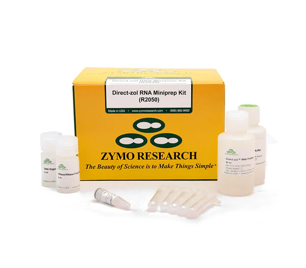
Figure 1.1: The Direct-zol<U+2122> RNA MiniPrep Kits are RNA purification kits that provide a streamlined method for the purification of up to 50 <U+00B5>g (per prep) of high-quality RNA directly from samples in TRI Reagent<U+00AE> or similar.
1.1.2 Library Preparation
The Direct RNA Sequencing Kit (SQK-RNA004) will be used to prepare and sequence isolated RNA. The preparation time is 135 minutes and inputs include 300 ng poly(A)+ RNA or 1 μg total RNA. This method does not require fragmentation or amplification, preserving long transcripts and RNA modifications. A description of the workflow is provided in Figure 1.2.
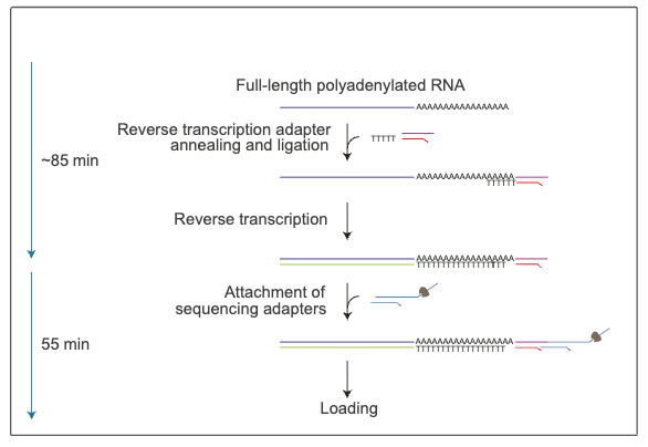
Figure 1.2: Starting from either total RNA or a poly(A)-enriched (poly(A)+) sample, adapters are ligated onto the RNA strand before a second complementary DNA (cDNA) strand is synthesised during reverse transcription. The cDNA strand is not sequenced but helps increase the sequencing output of native RNA molecules. Sequencing adapters are then attached to the RNA-cDNA hybrid.
1.1.3 Sequencing
Sequencing of direct RNA-seq libraries will be performed using the Oxford Nanopore PromethION 24 instrument (Figure 1.3). This is the highest output instrument that Oxford Nanopore produces. It has a total number of 24 independently controlled flow cells, meaning that the instrument can sequence up to 24 samples at once. Sample multiplexing is not currently supported for direct RNA-seq libraries. The sequencing provider that will be used for the NIRBA project has six PromethION 24 instruments.
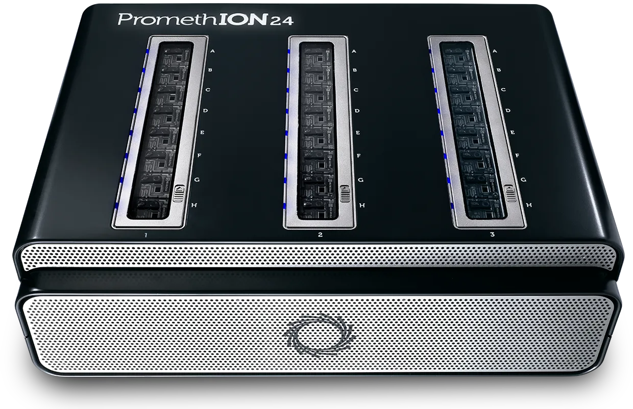
Figure 1.3: Oxford Nanopore PromethION 24 sequencing instrument
1.1.3.1 File Types
Nanopore sequencing data will be stored in the official POD5 format. Based on discussions with NIRBA and the ONT team, the expected output from each individual flow cell (or sample) is 700 GB. This implies that each sequencing run is expected to produce \(700 GB * 24 samples = 16,800 GB\) of nanopore sequencing data in POD5 format.
However, please be mindful of the fact that each flow cell has a theoretical maximum capacity of 2,030 GB, meaning that much more data could be produced. In my opinion, until a pilot experiment is completed, we can’t know for sure how much data will be produced by each flow cell - it could be more, it could be less. See Table 1 for example file sizes that could be produced based on different outputs from an individual flow cell.
Table 1. Example file sizes
| Flow cell output (Gbases) | POD5 storage (Gbytes) | FASTQ.gz storage (Gbytes) | Unaligned BAM with modifications (Gbytes) |
|---|---|---|---|
| 100 | 700 | 65 | 60 |
| 200 | 1,400 | 130 | 120 |
| 290 (TMO) | 2,030 | 188.5 | 174 |
1.1.3.2 Specifications
In addition to sequencing capabilities, the PromethION 24 instrument also has integrated compute and storage (see Table 2). In practice, this hardware is used to convert Nanopore sequence data in POD5 format into FASTQ or BAM files for downstream analysis, a process called basecalling (more on that later).
Unfortunately, the compute onboard the PromethION 24 instruments is not sufficient for basecalling this type and quantity of libraries. Indeed, internal testing by the ONT team revealed that each sample took between 24-28 hours to basecall, which becomes impractical when processing thousands of samples.
Table 2. PromethION 24 hardware specifications
| Component | Specification |
|---|---|
| Operating system | Ubuntu Focal (20.04) running off Intel CPU |
| Storage | 60 TB internal SSD |
| GPU cards | Data Acquisition Unit: 4× NVIDIA Ampere-series GPUs connected with NVLink |
| Memory | 512 GB RAM |
1.1.4 Key Considerations
1.1.4.1 RNA Integrity Number
The RNA Integrity Number (RIN) is a commonly used measure of RNA degradation, numbered between 1 (most degraded) and 10 (least degraded). Oxford Nanopore recommends isolated RNA to have a RIN ≥ 7 before proceeding with library preparation and sequencing. Indeed, the library RIN can have a direct impact on library yield, proportion of reads aligned to a reference genome, read length, and read N50 (Figure 1.4).
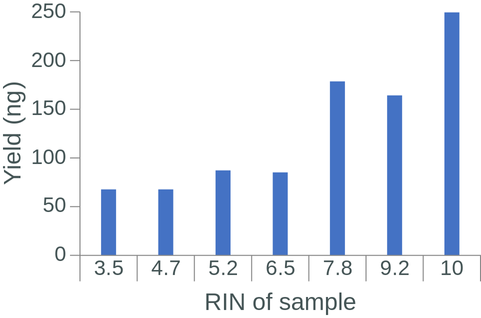
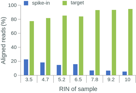
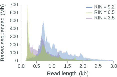
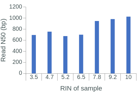
Figure 1.4: The effect of RIN on library yield, aligned reads, read length and read N50
1.1.4.2 Flow Cell Output
The total amount of sequencing data generated from an individual PromethION 24 flow cell is a function of RNA quality and instrument run time (Figure 1.5). We are expecting each flow cell to generate 700 GB of data per sample, but it does have the potential to generate more. This is important because it will have affect on storage costs if the data is archived with a commercial cloud provider. This includes the POD5 file and downstream outputs that get produced, such as BAM, BED and tertiary output files.
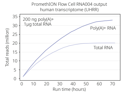
Figure 1.5: Flow cell output depends on RNA quality and instrument run time
1.1.4.3 Data Transfer
1.1.4.3.1 Option 1 (AWS Direct Connect)
The sequencing provider has a dedicated 10 Gbps network connection to AWS (AWS Direct Connect), allowing for fast and reliable transmission of POD5 files to the cloud. This is probably the most convenient solution for transferring petabytes of genomic data as it is an existing service feature. However, this does not mean that the network connection will be dedicated to the NIRBA project, so real transfer speeds could vary.
1.1.4.3.2 Option 2 (Hard Disks)
The sequencing provider can also distribute sequence data via hard disks. Indeed, this is a common practice for smaller sequencing projects, as most individual labs do not have experience working with commercial cloud providers like AWS. However, shipping clinical data via a hard disk may require additional encryption and a dedicated courier.
1.1.4.3.3 Option 3 (Dedicated Private Network Connection)
The sequencing provider does not have a dedicated private network connection that could be used to transfer genomic data to an external server (e.g., NUS server), but this is a functionality that the Oxford Nanopore team is open to working with NIRBA on. Both Equinix and SingAREN have been proposed as possible service providers. A final decision on where the sequence data is going and how it’s going to get there has not been made at this time.
1.2 Upstream Bioinformatics (POD5 to BAM)
1.2.1 Introduction
The primary output from an Oxford Nanopore sequencing device is a POD5 file. The POD5 file contains the raw signal traces measured by the device as genetic material passed through it. To be useful, the signal traces must be converted into a nucleotide sequence (ACGT), a process called basecalling.
Basecalling is performed using a command-line tool called Dorado. Dorado is a high-performance, easy-to-use and open-source basecaller for Oxford Nanopore reads written in the C++ programming language. It is maintained by Oxford Nanopore on GitHub and regularly updated with new features.
1.2.2 Basecalling Pipeline
The basecalling pipeline is split into several steps: data ingestion, basecalling, additional processing, sequence post-processing and writing. Each of these steps is described in more detail below.
1.2.2.1 Data Ingestion
The primary input to Dorado is a POD5 file. Legacy FAST5 files are not supported and must be converted to POD5 files if basecalling old data. This can be done using the pod5 python toolkit.
1.2.2.2 Basecalling
Basecalling is the process of converting raw signal traces into a human-readable nucleotide sequence (Figure 1.6). The process is computationally expensive and relies on specialized hardware devices called Graphical Processing Units (GPUs). Dorado is specifically optimized to run on NVIDIA A100 and H100 GPUs. If you are interested in learning more about basecalling speeds for different GPU architectures, please see this published benchmark.
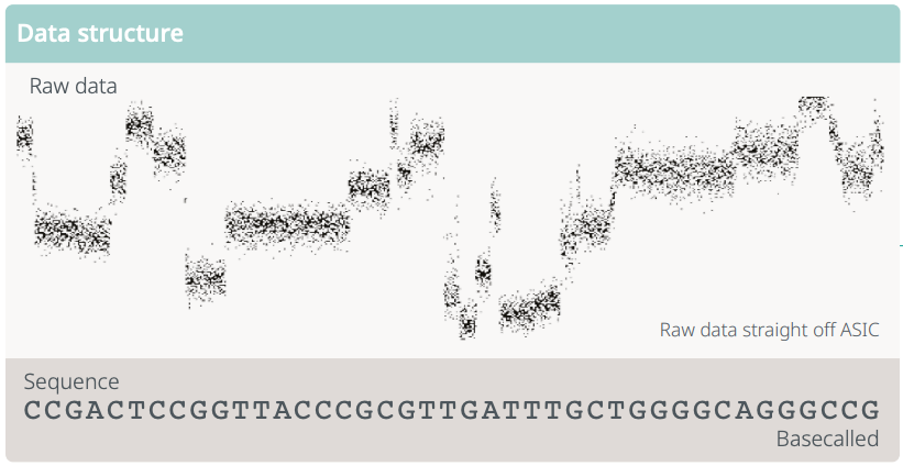
Figure 1.6: RNA passes through a nanopore, emitting an electrical signal. Machine learning algorithms are then used to convert the electrical signal into a sequence of RNA bases. This process is called basecalling.
To begin the basecalling process, a basecalling model must be selected. There are three flavors of basecalling models: fast, hac, and sup. The main difference between these three basecalling models is speed and accuracy (Figure 1.7).
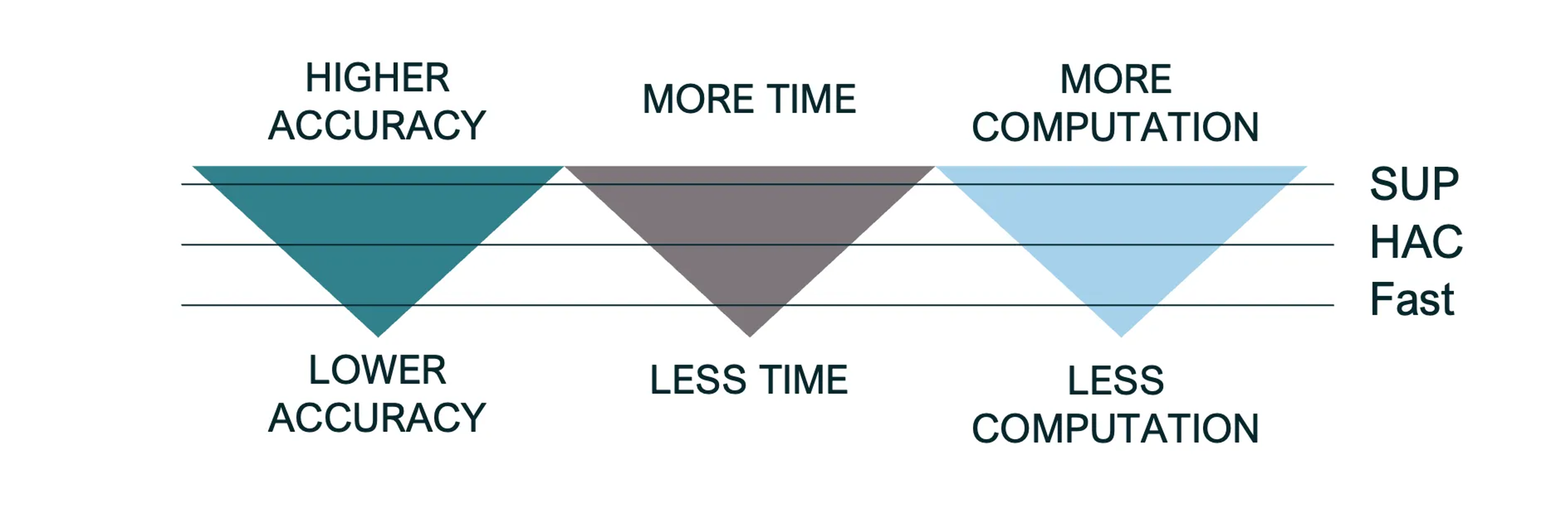
Figure 1.7: SUP models will result in the highest data quality, but require the most time and computation; Fast models will result in the lowest data quality, but require the least amount of time and computation; and HAC models offer a balance between the two.
Based on my personal communication with the Oxford Nanopore team in the U.S. and Singapore, the sup models are highly recommended for direct RNA-seq libraries. Indeed, these are the types of libraries that will be generated by NIRBA, so make sure to stick with the sup model.
1.2.2.3 Additional Processing (sequence alignment)
In addition to providing basecalling support, Dorado also allows users to align basecalled data to a reference genome or transcriptome. Sequence alignment is performed using the popular minimap2 aligner developed by Heng Li. This mode can be enabled by specifying the --reference <index> option and will produce an aligned BAM file.
When building the reference genome index, use the -x map-ont option in minimap2 for Oxford Nanopore reads. When performing the alignment within Dorado, further specify the --mm2-opts -ax splice -uf -k14 preset. These are the recommended indexing and alignment parameters for Oxford Nanopore direct RNA-seq libraries. A recent manuscript by Jonathan Göke’s group also used these presets for their dRNA-seq work (see Read alignment section under Methods).
1.2.2.4 Additional Processing (modification calling)
In addition to providing basecalling support of canonical bases (ACGT), Dorado also provides support for identifying base modifications. As of Dorado (v1.0.0), a total of eight RNA base modifications are supported (Table 3)
Table 3. Supported base modifications
| Model name | Full chemical name | Description |
|---|---|---|
| 2OmeG | 2′-O-methylguanosine (Gm) | Guanosine with a methyl group on the 2′-hydroxyl of the ribose. |
| m5C_2OmeC | 5-methylcytidine (m⁵C) + 2′-O-methylcytidine (Cm) | Detects 5-methylcytidine and 2′-O-methylcytidine. |
| inosine_m6A_2OmeA | Inosine (I) + N⁶-methyladenosine (m⁶A) + 2′-O-methyladenosine (Am) | Detects A→I editing, N⁶-methyladenosine, and 2′-O-methyladenosine. |
| pseU_2OmeU | Pseudouridine (Ψ) + 2′-O-methyluridine (Um) | Detects pseudouridylation and 2′-O-methyluridine. |
Modified base information will be stored in the optional fields of the BAM file (MM/ML tags). For more information about these optional fields, please see Section 1.7 of the SAM/BAM Format Specification.
Oxford Nanopore also provides a command-line tool called modkit to extract and summarize base modification calls from BAM files. The primary output from this tool is a bedMethyl file. The tool is CPU-intensive and can require a significant amount of RAM - hundreds of gigabytes - to process a single sample depending on the parameters used (e.g., modkit extract).
Another command-line tool called minimod was recently developed for base modification post-processing. The advantage of this tool is that it is vendor-agnostic, i.e., it works for both Oxford Nanopore and PacBio data. Indeed, both ONT and PacBio have their own base modification tools.
The advantage for NIRBA is that it is 54x times faster than modkit for RNA data. This is especially germane considering that modkit is quite slow in my experience (~3 hours to run a pileup from a 45GB BAM file). However, the disadvantage is that minimod is less feature rich and may not be actively maintained in the future without continued funding support.
Please note that Dorado does not provide a way to identify epigenetic modifications post-basecalling #1546. This means that this option must be specified at the time of basecalling if you want this information included in the BAM file. If new base modifications are released, then the entire basecalling pipeline will need to be rerun to capture them.
1.2.2.5 Sequence Post-Processing (poly A tail estimation)
Dorado also provides support for estimating poly(A)-tail lengths. This functionality can be enabled by setting the --estimate-poly-a option at the time of basecalling. Similar to base modification information, the estimated tail length is stored in the optional fields of the BAM file (pt:i and pa:B tags). More information about each of these tags can be found in the Dorado SAM specification.
Oxford Nanopore does not provide a tool for extracting and summarizing poly(A)-tail lengths, but setting the --emit-summary flag in Dorado will produce a read-level sequencing summary that extracts and summarizes this information. See the Sequencing Summary documentation for more information about this file.
Please note that Dorado does not provide a way to perform poly(A)-tail estimation post-basecalling #1475. This means that this option must be specified at the time of basecalling if you want this information included in the BAM file. Tools do exist for estimating poly(A)-tail lengths from the legacy FAST5 file format (see tailfindR and nanopolish), but not the POD5 file format.
1.2.3 Deliverables
| Deliverable | Description |
|---|---|
| BAM file | Contains all basecalls, associated quality scores, detected base modifications, and poly(A) tail length estimates for each read. |
| Sequencing summary | Provides read-level summary statistics, including identifiers, read lengths, quality metrics, and run-level performance indicators. |
1.3 Harmonized Datasets & Analysis Standards
This section provides a summary of the potential analyses and datasets that could be shared with NIRBA investigators.
1.3.1 Basecalling Datasets
1.3.1.2 QC Thresholds
I would not recommend performing any modifications to the basecalled reads before considering it production grade. The Dorado basecaller already removes reads shorter than 5bp #1190; long-read data is known to be inferior to that of short-reads with respect to quality, and that’s a tradeoff that should be accepted prior to generating the data.
1.3.1.3 Resource Dependencies
The Dorado basecalling pipeline relies heavilly on both CPU/GPU hardware. GPUs are primarily used for basecalling, modification calling and poly(A)-tail estimation; CPUs are primarily used for sequence alignment, adapter-trimming, and barcoder tasks #1498.
| Dataset | File Type | Tool | Description |
|---|---|---|---|
| Basecalled reads | BAM/CRAM | Dorado | Basecalled reads with quality scores, alignment info, base modifications |
| Index files | BAI/CRAI | SAMtools | Index files for BAM and CRAM files |
| Sequencing summary | TSV | Dorado | Read-level metadata including read length, quality scores, run metrics, and barcode info. |
1.3.2 Epigenetic Datasets
1.3.2.2 QC Thresholds
Base modifications are assigned a probability, similar to the way that a basecalled nucleotide is assigned a probability (i.e., Phred Quality Score). The recommended way to filter low confidence base modifications is to allow modkit to estimate a quality filtering threshold based on the input data.
In some cases, it is also recommended to inspect the base modification probabilities manually using the modkit sample-probs command to determine the appropriate filtering threshold. I would strongly recommend discussing this with Dr. Jonathan GÖKE as he has experience with this.
1.3.2.3 Resource Dependencies
Modkit is a CPU-intensive tool that can take quite a bit of time to run. The tool can also use a tremendous amount of memory depending on the paramters used (e.g., modkit extract), though there are ways to address this (see Performance Considerations).
| Dataset | File Type | Tool | Description |
|---|---|---|---|
| Per-base modification frequencies | bedMethyl | modkit pileup | Summary counts of modified and unmodified bases. |
| Read-level base modification calls | bedMethyl | modkit extract calls | Table of read-level base modification calls. |
| Read-level statistics | TSV | modkit modbam summary | Read-level statistics on either a sample of reads, a region, or an entire BAM. |
1.3.3 Quantification Datasets
1.3.3.1 Pipeline
Transcript and gene quantifications can be calculated directly from the aligned BAM files using several tools: Bambu, NanoCount or Salmon. I would recommend generating separate transcript and gene quantifications using each tool in the case that someone has a preference. Transcript and gene quantifications can then be normalized using transcripts per million (TPM) and counts per million (CPM), respectively.
1.3.3.2 QC Thresholds
I would not recommend applying any quality control filters to the raw or normalized counts even if there are genetic features with few or no counts across samples. The presence of few or the absence of features in a sample or experimental group is still a result and may be relevant to someone depending on their research question.
1.3.3.3 Resource Dependencies
Gene and transcript quantification tools utilize CPUs and typically have minimal resource requirements. Batching samples prior to quantification is not required; however, tools like Bambu can benefit from batching when performing a comparative analysis, e.g., when the goal is to compare expression between experimental groups, because novel transcripts will be given the same identifier, which is useful for differential expression analyses. For more information about this, please see the Running Multiple Samples section from the Bambu documentation.
| Dataset | File Type | Tool | Description |
|---|---|---|---|
| Gene counts | TSV | Bambu, Nanocount, Salmon | Raw gene counts |
| Transcript counts | TSV | Bambu, Nanocount, Salmon | Raw transcript counts |
| Gene counts per million | TSV | R | CPM normalized gene counts |
| Transcripts per million | TSV | R | TPM normalized transcript counts |